Applications of BFS
Published on 2018-05-07
The breadth-first search algorithm (BFS) is one of the most widely used algorithms in graph theory, and it can be applied to a variety of problems and tasks. As we shall see in this post, some of these problems are not initially presented in the form of a graph, but they can be transformed into graph theory problems so they can be solved more efficiently.
Some applications of BFS
One group of problems that is not initially presented in the form of a graph, but which may be solved with graph theory algorithms, are those problems that start with a set of possible objects or states (locations, integers, tennis balls, etc.), and a list of operations that can be used to go from one state to another. Now, let's say that we want to calculate the minimum number of operations that need to be executed to get from an initial state to an end state. In tasks like this, we can represent the problem using a graph, and use the BFS algorithm to calculate the number of operations.
For example, let's start from one number (for example, N=10), and say that we want to reach some other number (for example, R=63). Also, we have a list of operations that we can perform on a given number, and those operations are: "multiplication by 2", "multiplication by 3", and "adding the value 1, i.e, incrementing by 1". Then, we can go from the number N=10 to R=63 with 3 operations: first multiply by 2 to reach 10*2=20, then add 1 to reach 20+1=21, and finally multiply by 3 to reach 21*3=63. The number 63 cannot be reached with less than 3 operations. But, how can we write an algorithm, so that our computer can solve this problem for any N and R?
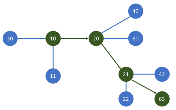
The solution is simple, and it comes down to the following idea: we can represent the numbers as vertices (in a graph), and represent the operations as edges through which we can travel from one vertex (for example, 10) to another (30). Since the breadth-first search algorithm will visit the vertices that are closest to the starting vertex first, it will also get to the final vertex by traveling the least number of edges (which in our case is basically the smallest number of operations). However, please remember that the BFS algorithm only works in cases where all edges have equal weight/length - so, for example, this algorithm will not calculate the correct answer if the edges (or in our case, the operations to move from one number to another) are weighted differently - i.e. we must be solving a problem of finding the minimum number of operations where each of them counts as 1. Specifically, the BFS algorithm treats all neighbors of one vertex as equal (without giving preference to those where the edge length is smaller, or where an operation has the lowest cost).
Let's go back to discussing our problem and the breadth-first search algorithm - since it can be applied to various other problems as well (including ours, because the edges in our graph have the same weight, or we can think of them as having a weight of 1). As we already said, the main obstacle to solving the original problem is noticing that we can represent it using a graph. Afterwards, we just need to use the BFS algorithm. There is no need to represent the edges in the graph directly (with an adjacency list or a matrix). Instead, we can create the edges by looking at each of the numbers in our BFS queue (for example, if the number which we are currently looking at is 10, then the next vertices will be 10*2, 10*3, and 10+1), because the permitted operations in our case are multiplication by 2, multiplication by 3, and incrementing by 1. Let's see how the source code looks like:
#include <iostream>
#include <queue>
#include <cstring>
using namespace std;

vector<int> possible_operations(int node)
{

     vector<int> moves;
     moves.push_back(node*2);
     moves.push_back(node*3);
     moves.push_back(node+1);

     return moves;
}

int BFS(int N, int R)
{

     queue<int> queue;


     int operations[R + 1];
     memset(operations, 127, sizeof(operations)); //some large number

     queue.push(N);
     operations[N] = 0;   //0 operations are needed to reach N (start)

     while (!queue.empty())
     {
          auto node = queue.front();
          queue.pop();

          if (node == R)
          {
               //we discovered the answer
               break;
          }

          vector<int> moves = possible_operations(node);

          for (auto next : moves)
          {
               if (next <= R)     //we don't look at numbers larger than R
               {
                    if (operations[next] > operations[node] + 1)
                    {
                         //we can go from "node" to "next" in 1 operation
                         operations[next] = operations[node] + 1;
                         queue.push(next);
                    }
               }
          }
     }

     return operations[R];
}


int main()
{

     int N, R;
     cout << "Please enter N and R (make sure R>N): " << endl;
     cin >> N >> R;

     int minOperations = BFS(N, R);
     cout << minOperations << endl;
     return 0;
}
A pretty short and readable source code, but it shows us how to use the breadth-first search algorithm to solve a variety of problems. For example, imagine that you are employed in a company working on software that will tackle math problems, and you want to write a program that will solve tasks by using the minimum number of steps. More specifically, if we can define the operations that can be applied to an equation, then the software will be able to solve a variety of equations very quickly - meaning that it can be used by students to check their homework, etc. In our graph, the vertices will represent the equations, and the edges will represent the operations through which we can go from one equation to another, as shown below.
2x + 3 = 5 – 6 (vertex 1, start)
2x = 5 – 6 – 3 (vertex 2, reached from vertex 1, by subtracting 3 on both sides)
2x = -4 (vertex 3, reached from vertex 2, by calculating the value on the right side)
x = -2 (vertex 4, reached from vertex 3, by dividing both sides by 2)
Shortest path in a maze
Finding the shortest path in a maze is a common example of using the breadth-first search algorithm, because these problems are often encountered in computer games, robotics, and other similar fields. First, let's define the problem that we want to solve. Let's imagine that we have been given a matrix as shown in the picture below, which contains some fields (marked with a white background) through which we can move, and other fields (marked in gray) through which we can't move (let's call them obstacles). If we also have two locations in the matrix (start and finish), can we write a program that will find the shortest path from the start location to the finish (as the number of movements that need to be made between adjacent fields), without stepping on obstacles? On the right side of the picture, you can see the shortest path between the starting location (S) and the finish (E).
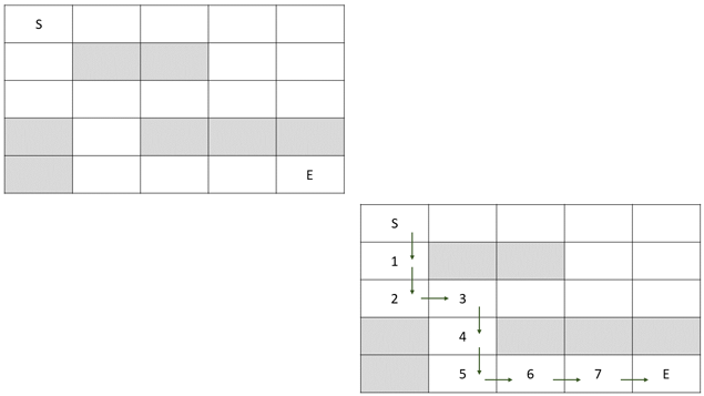
This problem can be solved by using the breadth-first search (BFS) algorithm. Specifically, as we mentioned before, this algorithm visits the vertices (in our case, these are the fields in the matrix) by first looking at the ones closest to the start. If we store the distance to a vertex as we visit it (i.e. how many fields we should go through in order to reach it), then the numbers written in each field will correspond exactly to the required minimum number of steps needed to reach those locations.
Before we look at the implementation of this solution, let's note a few more things. When we look at a certain vertex (field in the matrix), we immediately know the vertices that are adjacent to it: those that lie next to it in the matrix. In other words, there is no need to define adjacency lists G[i], where a list stores the edges of the vertex i, etc. Instead, if we imagine that we're currently at location (row 3, column 4), for example, then the adjacent fields are those next to it: up (row 2, column 4), down (row 4, column 4), left (row 3, column 3), etc. Depending on whether or not we can move diagonally, or just horizontally and vertically, there will be 8 adjacent vertices (if diagonal movement is allowed), or 4.
The last note we want to make is that we'll use just one matrix to store all the data (the input, distance to a vertex, etc). Specifically, while reading the data, we can use a matrix of the appropriate size to represent the maze, and then use certain numbers to denote the corresponding fields (mark the starting field with 0, mark the obstacles with -1, mark every other field with it's distance from the starting location - 1, 2, 3, etc.). Similarly, there is no need to create a separate array in order to store which vertices have already been visited (as it's often done with BFS), because this data can be read from the matrix itself. However, if we really want to (i.e. if it's easier to reason that way), we can use such an array.
#include <iostream>
#include <queue>
using namespace std;


//we use 999999 (a large value) to mark
//fields we haven't visited (yet)
int rows = 5, cols = 5;
int labyrinth[5][5] =
{
     { 0,        999999,  999999,    999999,   999999 },
     { 999999,    -1,       -1,      999999,   999999 },
     { 999999,   999999,  999999,    999999,   999999 },
     { -1,       999999,    -1,       -1,      -1     },
     { -1,       999999,  999999,    999999,   999999 }
};


//the starting location and the finish are usually given upfront;
//in this example, start is at (0, 0), and finish is at (4, 4)
//if you look at the matrix above, start is on top-left
int start_row = 0, start_col = 0;
int end_row   = 4,   end_col = 4;


//check if a field is valid
bool valid_move(pair<int, int> next)
{

     //valid if inside the matrix (can't go out), and no obstacle
     return (next.first >= 0 && next.first < rows
          && next.second >= 0 && next.second < cols
          && labyrinth[next.first][next.second] != -1);
}

vector<pair<int, int> > possible_moves(pair<int, int> node)
{

     vector<pair<int, int> > moves;
     moves.push_back({node.first, node.second - 1}); //left
     moves.push_back({node.first, node.second + 1}); //right
     moves.push_back({node.first - 1, node.second}); //up
     moves.push_back({node.first + 1, node.second}); //down

     //if diagonal movement is allowed
     //moves.push_back({node.first - 1, node.second - 1});
     //moves.push_back({node.first - 1, node.second + 1});
     //moves.push_back({node.first + 1, node.second - 1});
     //moves.push_back({node.first + 1, node.second + 1});

     return moves;
}


int BFS()
{

     queue<pair<int, int> > queue;
     queue.push({start_row, start_col});

     while (!queue.empty())
     {
          auto node = queue.front();
          queue.pop();

          vector<pair<int, int> > moves = possible_moves(node);

          for (auto next : moves)
          {
               if (valid_move(next))
               {
                    if (labyrinth[next.first][next.second] == 999999)
                    {
                         //field not visited yet
                         queue.push(next);

                         int distance = labyrinth[node.first][node.second] + 1;
                         labyrinth[next.first][next.second] = distance;
                    }
               }
          }
     }
}


int main()
{

     BFS();

     int distance = labyrinth[end_row][end_col];
     cout << distance << endl;
}
Note that we use a queue, look at the vertices one after another, etc - all standard BFS. When we discover a new unvisited field, we store the distance in the matrix, as it is equal to the distance of the vertex we used to get to it, plus 1.
When we look at a field and want to find out which neighbours we can go to, we use the function possible_moves(). Of course, it is also necessary to check that those fields are valid - whether they are inside the matrix or perhaps outside (for example, the field [-1, 3] is invalid, because the row -1 does not exist). Additionally, we also need to be careful not to step on an obstacle (marked with -1 in the matrix).
Often, when solving such problems, the size of the matrix and the elements in it will be given to us as input, rather than being directly coded into the program. In the example given above, the data was part of the source code so that it's easier to play with. Of course, only minimal changes are needed to read this data from standard input or file (cin >> rows >> cols, cin >> start_row >> start_col, etc.).
The time complexity of the algorithm given above is O(V), since the complexity of the BFS algorithm is O(V + E), and the number of edges in our case is directly dependent on the number of vertices - x4 if we do not allow diagonal movement (or x8, if such movement is allowed). When we do time complexity analysis we throw out all constant factors (in this case, V + 4V = 5V), so we conclude that the algorithm has linear time complexity O(V). Otherwise, if we want to, we can analyze the complexity a bit further, and see that the number of vertices V is equal to the size of the matrix (number of rows * number of columns), so we can also say that the complexity is O(R * C).
Some final thoughts
In this post, we looked at several applications of graph theory, by focusing on the breadth-first search algorithm (BFS). BFS can be used to explore edges in a graph, to find the shortest path in a maze (where all edges, i.e. movements from one vertex to another have weight 1), to find the minimal number of operations required to go from one state to another, etc. It is very important to have an extra array/map (or matrix) where we store which vertices have already been visited, or to store the distance. This is of great importance in graph theory algorithms, because there is often a way to travel in the opposite direction (from one vertex to another, and vice versa), so we do not want to get stuck in a loop and reach a situation where we look at the same vertices all the time.